The core R language is extended by a large number of software packages, which contain reusable code, documentation, and sample data. Some of the most popular R packages are in the tidyverse collection, which enhances functionality for visualizing, transforming, and modelling data, as well as improves the ease of programming (according to the authors and users).[10]
The name of the language, R, comes from being both an S language successor and the shared first letter of the authors, Ross and Robert.[13] In August 1993, Ihaka and Gentleman posted a binary file of R on StatLib — a data archive website.[14] At the same time, they announced the posting on the s-news mailing list.[15] On 5 December 1997, R became a GNU project when version 0.60 was released.[16] On 29 February 2000, the 1.0 version was released.[17]
Immediately available when starting R after installation, base packages provide the fundamental and necessary syntax and commands for programming, computing, graphics production, basic arithmetic, and statistical functionality.[21]
An example is the tidyverse collection of R packages, which bundles several subsidiary packages to provide a common API. The collection specializes in tasks related to accessing and processing "tidy data",[22] which are data contained in a two-dimensional table with a single row for each observation and a single column for each variable.[23]
Installing a package occurs only once. For example, to install the tidyverse collection:[23]
> install.packages("tidyverse")
To load the functions, data, and documentation of a package, one calls the library() function. To load the tidyverse collection, one can execute the following code:[a]
> # The package name can be enclosed in quotes> library("tidyverse")> # But the package name can also be used without quotes> library(tidyverse)
The R Consortium is one of the three main groups that support R
There are three main groups that help support R software development:
The R Core Team was founded in 1997 to maintain the R source code.
The R Foundation for Statistical Computing was founded in April 2003 to provide financial support.
The R Consortium is a Linux Foundation project to develop R infrastructure.
The R Journal is an open access, academic journal that features short to medium-length articles on the use and development of R. The journal includes articles on packages, programming tips, CRAN news, and foundation news.
UseR! conference is one place the R community can gather at
The R community hosts many conferences and in-person meetups.[b] These groups include:
UseR!: an annual international R user conference (website)
Directions in Statistical Computing (DSC) (website)
Here is an alternative version, which uses the cat() function:
> cat("Hello, World!")Hello, World!
Basic syntax
The following examples illustrate the basic syntax of the language and use of the command-line interface.[c]
In R, the generally preferred assignment operator is an arrow made from two characters <-, although = can be used in some cases.[32]
> x<-1:6# Create a numeric vector in the current environment> y<-x^2# Similarly, create a vector based on the values in x.> print(y)# Print the vector’s contents.[1] 1 4 9 16 25 36> z<-x+y# Create a new vector that is the sum of x and y> z# Return the contents of z to the current environment.[1] 2 6 12 20 30 42> z_matrix<-matrix(z,nrow=3)# Create a new matrix that transforms the vector z into a 3x2 matrix object> z_matrix [,1] [,2][1,] 2 20[2,] 6 30[3,] 12 42> 2*t(z_matrix)-2# Transpose the matrix; multiply every element by 2; subtract 2 from each element in the matrix; and then return the results to the terminal. [,1] [,2] [,3][1,] 2 10 22[2,] 38 58 82> new_df<-data.frame(t(z_matrix),row.names=c("A","B"))# Create a new dataframe object that contains the data from a transposed z_matrix, with row names 'A' and 'B'> names(new_df)<-c("X","Y","Z")# Set the column names of the new_df dataframe as X, Y, and Z.> print(new_df)# Print the current results. X Y ZA 2 6 12B 20 30 42> new_df$Z# Output the Z column[1] 12 42> new_df$Z==new_df['Z']&&new_df[3]==new_df$Z# The dataframe column Z can be accessed using the syntax $Z, ['Z'], or [3], and the values are the same. [1] TRUE> attributes(new_df)# Print information about attributes of the new_df dataframe$names[1] "X" "Y" "Z"$row.names[1] "A" "B"$class[1] "data.frame"> attributes(new_df)$row.names<-c("one","two")# Access and then change the row.names attribute; this can also be done using the rownames() function> new_df X Y Zone 2 6 12two 20 30 42
Structure of a function
R is able to create functions that add new functionality for code reuse.[33]Objects created within the body of the function (which are enclosed by curly brackets) remain accessible only from within the function, and any data type may be returned. In R, almost all functions and all user-defined functions are closures.[34]
The following is an example of creating a function to perform an arithmetic calculation:
# The function's input parameters are x and y.# The function, named f, returns a linear combination of x and y.f<-function(x,y){z<-3*x+4*y# An explicit return() statement is optional--it could be replaced with simply `z` in this case.return(z)}# As an alternative, the last statement executed in a function is returned implicitly.f<-function(x,y)3*x+4*y
The following is some output from using the function defined above:
Since R version 4.1.0, functions can be written in a short notation, which is useful for passing anonymous functions to higher-order functions:[35]
> sapply(1:5,\(i)i^2)# here \(i) is the same as function(i) [1] 1 4 9 16 25
Native pipe operator
In R version 4.1.0, a native pipe operator, |>, was introduced.[36] This operator allows users to chain functions together, rather than using nested function calls.
> nrow(subset(mtcars,cyl==4))# Nested without the pipe character[1] 11> mtcars|>subset(cyl==4)|>nrow()# Using the pipe character[1] 11
Another alternative to nested functions is the use of intermediate objects, rather than the pipe operator:
While the pipe operator can produce code that is easier to read, it is advisable to chain together at most 10-15 lines of code using this operator, as well as to chunk code into sub-tasks that are saved into objects having meaningful names.[37]
The following is an example having fewer than 10 lines, which some readers may find difficult to grasp in the absence of intermediate named steps:
The R language has native support for object-oriented programming. There are two native frameworks, the so-called S3 and S4 systems. The former, being more informal, supports single dispatch on the first argument, and objects are assigned to a class simply by setting a "class" attribute in each object. The latter is a system like the Common Lisp Object System (CLOS), with formal classes (also derived from S) and generic methods, which supports multiple dispatch and multiple inheritance[38]
In the example below, summary() is a generic function that dispatches to different methods depending on whether its argument is a numeric vector or a factor:
> data<-c("a","b","c","a",NA)> summary(data) Length Class Mode 5 character character > summary(as.factor(data)) a b c NA's 2 1 1 1
Modeling and plotting
Diagnostic plots for the model from the example code in the "Modeling and plotting" section (q.v. the plot.lm() function). Mathematical notation is allowed in labels, as shown in the lower left plot.
The R language has built-in support for data modeling and graphics. The following example shows how R can generate and plot a linear model with residuals.
# Create x and y valuesx<-1:6y<-x^2# Linear regression model: y = A + B * xmodel<-lm(y~x)# Display an in-depth summary of the modelsummary(model)# Create a 2-by-2 layout for figurespar(mfrow=c(2,2))# Output diagnostic plots of the modelplot(model)
The output from the summary() function in the preceding code block is as follows:
Residuals: 1 2 3 4 5 6 7 8 9 10 3.3333 -0.6667 -2.6667 -2.6667 -0.6667 3.3333Coefficients: Estimate Std. Error t value Pr(>|t|) (Intercept) -9.3333 2.8441 -3.282 0.030453 * x 7.0000 0.7303 9.585 0.000662 ***---Signif. codes: 0 ‘***’ 0.001 ‘**’ 0.01 ‘*’ 0.05 ‘.’ 0.1 ‘ ’ 1Residual standard error: 3.055 on 4 degrees of freedomMultiple R-squared: 0.9583, Adjusted R-squared: 0.9478F-statistic: 91.88 on 1 and 4 DF, p-value: 0.000662
Mandelbrot set
A Mandelbrot set as visualized in R. (Note: The colours in this image differ from the output of the sample code in the "Mandelbrot set" section.)
To run this sample code, it is necessary to first install the package that provides the write.gif() function:
install.packages("caTools")
The sample code is as follows:
library(caTools)jet.colors<-colorRampPalette(c("green","pink","#007FFF","cyan","#7FFF7F","white","#FF7F00","red","#7F0000"))dx<-1500# define widthdy<-1400# define heightC<-complex(real=rep(seq(-2.2,1.0,length.out=dx),each=dy),imag=rep(seq(-1.2,1.2,length.out=dy),times=dx))# reshape as matrix of complex numbersC<-matrix(C,dy,dx)# initialize output 3D arrayX<-array(0,c(dy,dx,20))Z<-0# loop with 20 iterationsfor (kin1:20){# the central difference equationZ<-Z^2+C# capture the resultsX[,,k]<-exp(-abs(Z))}write.gif(X,"Mandelbrot.gif",col=jet.colors,delay=100)
Version names
A CD of R Version 1.0.0, autographed by the core team of R, photographed in Quebec City in 2019
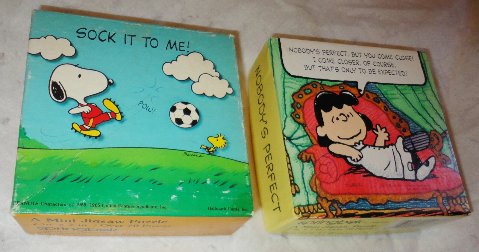
All R version releases from 2.14.0 onward have codenames that make reference to Peanuts comics and films.[39][40][41]
In 2018, core R developer Peter Dalgaard presented a history of R releases since 1997.[42] Some notable early releases before the named releases include the following:
Version 1.0.0, released on 29 February 2000, a leap day
Version 2.0.0, released on 4 October 2004, "which at least had a nice ring to it"[42]
The idea of naming R version releases was inspired by the naming system for Debian and Ubuntu versions. Dalgaard noted an additional reason for the use of Peanuts references in R codenames—the humorous observation that "everyone in statistics is a P-nut."[42]
^This code displays to standard error a listing of all the packages that the tidyverse collection depends upon. The code may also display warnings showing namespace conflicts, which may typically be ignored.
^ abHornik, Kurt; The R Core Team (12 April 2022). "R FAQ". The Comprehensive R Archive Network. 3.3 What are the differences between R and S?. Archived from the original on 28 December 2022. Retrieved 27 December 2022.
^Chambers, John M. (2020). "S, R, and Data Science". The R Journal. 12 (1): 462–476. doi:10.32614/RJ-2020-028. ISSN2073-4859. The R language and related software play a major role in computing for data science. ... R packages provide tools for a wide range of purposes and users.
^Davies, Tilman M. (2016). "Installing R and Contributed Packages". The Book of R: A First Course in Programming and Statistics. San Francisco, California: No Starch Press. p. 739. ISBN9781593276515.
^Talbot, Justin; DeVito, Zachary; Hanrahan, Pat (1 January 2012). "Riposte: A trace-driven compiler and parallel VM for vector code in R". Proceedings of the 21st international conference on Parallel architectures and compilation techniques. ACM. pp. 43–52. doi:10.1145/2370816.2370825. ISBN9781450311823. S2CID1989369.


.jpg)


.png)


